Now that you have loaded your FIA data into R, it’s time to put it to work. Let’s explore the basic functionality of rFIA with tpa, a function to compute tree abundance estimates (TPA, BAA, & relative abundance (%)) from FIA data, and fiaRI, a subset of the FIA Database for Rhode Island including all inventories from 2014-2018.
rFIA. Copy and paste the code below into R to follow along!
Spatial and temporal queries
Are you only interested in producing estimates for a specific inventory year or within a portion of your state? clipFIA allows you to easily query (subset) your FIA.Database object so you only use the data you need. This will conserve RAM on your machine and speed processing time.
Load some data
## Load rFIA package
library(rFIA)

## Load some data
data('fiaRI')
data('countiesRI')
Most recent subsets
To subset only the data needed to produce estimates for the most recent inventory year (2017 in our case), users can simply pass their FIA.Database object to clipFIA, or more explicitly specify mostRecent = TRUE in the call:
## Most Recent Subset (2017)
riMR <- clipFIA(fiaRI)

# More explicity (identical to above)
riMR <- clipFIA(fiaRI, mostRecent = TRUE)
Spatial subsets
To subset the data required to produce estimates within an user-defined areal region (should be contained within the spatial extent of the FIA.Database object), simply pass a spatial polygon object (from sp or sf packages) to the mask argument of clipFIA. In our example below, the spatial subset does little to reduce the size of our FIA.Database object, although the effect is likely to be much more substantial if applied to larger state or region.
## Select Kent County RI
kc <- countiesRI[2,] ## SF Multipolygon object

## Subset the data
riKC <- clipFIA(fiaRI, mask = kc, mostRecent = FALSE)

## Most recent subset, within Kent County
riKC <- clipFIA(fiaRI, mask = kc)
Basic population estimates
To produce tree abundance estimates and associated sampling errors for the state of Rhode Island, simply hand your FIA.Database object to the db argument of tpa():
## TPA & BAA for the most recent inventory year
tpaRI_MR <- tpa(riMR)

## All Inventory Years Available (i.e., returns a time series)
tpaRI <- tpa(fiaRI)
totals = TRUE in the call to tpa. If you do not want to estimate sampling errors, specify SE = FALSE (often much faster).
Basic plot-level estimates
To return the same estimates at the plot level (e.g., mean TPA & BAA for each plot), specify byPlot = TRUE. For subplot or tree-level estimates, specify byPlot = TRUE and grpBy = SUBP or grpBy = TREE, respectively:
## Plot-level
tpaRI_plot <- tpa(riMR, byPlot = TRUE)

## Subplot-level
tpaRI_subp <- tpa(riMR, byPlot = TRUE, grpBy = SUBP)

## Tree-level
tpaRI_tree <- tpa(riMR, byPlot = TRUE, grpBy = TREE)
Grouping by species and size class
What if I want to group estimates by species? How about by size class? Easy! Just specify bySpecies and/ or bySizeClass as TRUE in the call to tpa. By default, estimates are returned within 2 inch size classes, but you can make your own size classes using makeClasses!
## Group estimates by species
tpaRI_species <- tpa(riMR, bySpecies = TRUE)

## Group estimates by size class
tpaRI_sizeClass <- tpa(riMR, bySizeClass = TRUE)

## Group by species and size class, and plot the distribution
tpaRI_spsc <- tpa(riMR, bySpecies = TRUE, bySizeClass = TRUE)
Grouping by other variables
To group estimates by a variable defined the FIA Database (other than species or size class), pass the variable name to the grpBy argument of tpa. You can find definitions of all variables in the FIA Database in the the FIA User Guide. Variables of interest will most likely be contained in the condition (COND), plot (PLOT), or tree (TREE) tables.
## grpBy specifies what to group estimates by (just like species and size class above)
## NOTICE the variable names passed to grpBy are NOT quoted

# Ownership Group
tpaRI_own <- tpa(riMR, grpBy = OWNGRPCD)

# Ownership Group (for all available inventories)
tpaRI_ownAll <- tpa(fiaRI, grpBy = OWNGRPCD)

# Site Productivity Class
tpaRI_spc <- tpa(riMR, grpBy = SITECLCD)

# Forest Type
tpaRI_ft <- tpa(riMR, grpBy = FORTYPCD)

## Combining multiple grouping variables: Site Productivity within Forest Types
tpaRI_ftspc <- tpa(riMR, grpBy = c(FORTYPCD, SITECLCD))
grpBy should NOT be quoted. Multiple grouping variables should be combined with c(), and grouping will occur hierarchically. For example, to produce separate estimates for each ownership group within ecoregion subsections, specify c(ECOSUBCD, OWNGRPCD).
Unique areas or trees of interest
Do you want estimates for a specific type of tree (e.g., greater than 12-inches DBH and in a canopy dominant or subdominant position) in specific area (e.g., growing on mesic sites)? Each of these specifications are described in the FIA Database, and all rFIA estimator functions can leverage these data to easily implement complex queries!
For a conditions related to trees of interest (e.g., diameter, height, crown class, etc.) pass a logical statement to treeDomain. For conditions related to area(e.g., ecoregions, counties, forest types, etc.), pass a logical statement to areaDomain. These statements should NOT be quoted.
## Estimate abundance of trees greater than 12-inches DBH in a dominant
## or subdominant canopy position growing on mesic sites
tpaRI_domain <- tpa(riMR,
                 treeDomain = DIA > 12 & CCLCD %in% c(1,2),
                 areaDomain = PHYSCLCD %in% 20:29)

## In the code above, DIA describes the DBH of stems,
## CCLCD thier canopy position, and PHYSCLCD the
## physiographic class upon which the class occurs
Visualization
Now that we have produced some estimates, we should translate them into plots so we can easily see the status and trends in our selected forest attributes. Using plotFIA, we can easily produce (1) simple or grouped time series plots, (2) simple or grouped plots with a user defined x-axis (e.g., size class), and (3) spatial choropleth maps (see Incorporating Spatial Data).
Time Series Plots
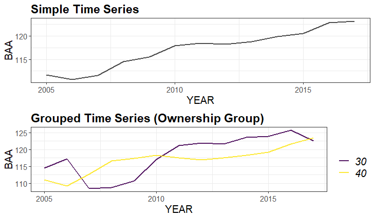
By default, plotFIA will produce time series plots if you produced estimates for more than one reporting year and do not specify a non-temporal x-axis. To produce a grouped time series, simply hand the grouping variables to the grp argument of plotFIA (should correspond with the grpBy argument of estimating function).
## Using our estimates from above (all inventory years in RI)
plotFIA(tpaRI, y = BAA, plot.title = 'Simple Time Series')

## Grouped time series by ownership class
plotFIA(tpaRI_ownAll, y = BAA, grp = OWNGRPCD, plot.title = 'Grouped Time Series (Ownership Group)')
Non-temporal plots
To define your own x-axis, simply specify the variable you would like to use in the x argument of the plotFIA call. This is great for plotting things like size-class distributions. Since these plots do not have time as axis, they are best suited for plotting estimates from a single point in time (e.g., a most recent subset).
## Using our estimates from above (all inventory years in RI)
plotFIA(tpaRI_sizeClass, y = BAA, x = sizeClass, plot.title = 'Simple size class distribution')

## Grouped time series by ownership class
plotFIA(tpaRI_spsc, y = BAA, grp = COMMON_NAME, x = sizeClass, n.max = 5, plot.title = 'Grouped size class distribution')
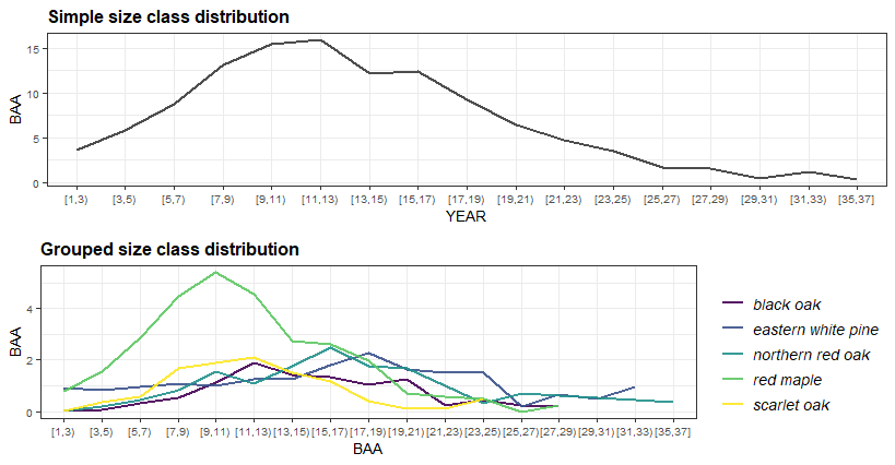
n.max to any grouped call to plotFIA to only display the top or bottom n groups in your plot. In the call above we specified n.max = 5, resulting in the species with the highest average basal area per acre values being plotted. To only plot the bottom five, specify n.max = -5.
Variance vs Sampling Error
FIA’s flagship online estimation tools, EVALIDator, reports estimates of uncertainty as “% sampling error” (SE). While the definition is a bit elusive, this measure is simply the % coefficient of variation, or the sample standard deviation divided by the sample mean multiplied by 100. FIA opts to report SE as opposed to sample variance because SE provides an easy, “standardized” way to compare uncertainty across estimates with very different absolute values (i.e., how large is the “spread” relative to the mean?). However, SE has its downsides. First, confidence intervals cannot be derived directly from SE. Second, the “standardized” nature of the SE breaks down as the mean approaches zero (SE approaches infinity in this case), making it particularly uninformative for change estimates that tend near zero.
In rFIA we allow users to return estimates of uncertainty in terms of SE or sample variance using the variance argument (where variance=TRUE returns sample variance and sample size). Along with sample size, sample variance can be used to produce proper confidence intervals for totals and ratios:
## TPA with % sampling error (SE)
tpaSE <- tpa(riMR, variance = FALSE)
tpaSE
## # A tibble: 1 x 8
##    YEAR   TPA   BAA TPA_SE BAA_SE nPlots_TREE nPlots_AREA     N
##   <int> <dbl> <dbl>  <dbl>  <dbl>       <int>       <int> <int>
## 1  2018  427.  122.   6.63   3.06         126         127   199
## TPA with % sampling error (SE)
tpaVAR <- tpa(riMR, variance = TRUE)
tpaVAR
## # A tibble: 1 x 8
##    YEAR   TPA   BAA TPA_VAR BAA_VAR nPlots_TREE nPlots_AREA     N
##   <int> <dbl> <dbl>   <dbl>   <dbl>       <int>       <int> <int>
## 1  2018  427.  122.    801.    13.9         126         127   199
## Estimate 95% confidence interval around 2018 TPA
halfInt <- qt(0.975, tpaVAR$N - 1) * sqrt(tpaVAR$TPA_VAR)

## Lower
tpaVAR$TPA - halfInt
## [1] 370.9086
## Upper
tpaVAR$TPA + halfInt
## [1] 482.5153
\(t_{n-1} \frac{\sigma}{\sqrt{N}}\)), as opposed to sample totals and ratios (i.e., \(t_{n-1} \sigma\)). This was incorrect for the above application, and for nearly all applications of FIA’s design-based estimators. The above example exhibits the correct CI formula for most applications involving FIA (i.e., involving design-based estimators of totals and/or ratios).
Other rFIA functions
Fortunately, all of the rFIA estimator functions are structured in the same way as tpa. Therefore you can use essentially the same argument calls we’ve used above to produce estimates of other types of forest attributes!
In the table below we list the availability of the argument calls we have explored in the examples above for all rFIA estimator functions. In some cases, like that of dwm (estimates of down woody material volume, biomass & carbon) it does not make sense to include arguments like treeDomain or bySpecies, and hence these arguments are unavailable.
rFIA Function |
bySpecies | bySizeClass | treeDomain | areaDomain | tidy |
|---|---|---|---|---|---|
biomass |
+ | + | + | + | - |
carbon |
- | - | + | + | - |
diversity |
- | + | + | + | - |
dwm |
- | - | - | + | + |
growMort |
+ | + | + | + | - |
invasive |
(default) | - | - | + | - |
standStruct |
- | - | - | + | + |
tpa |
+ | + | + | + | - |
vitalRates |
+ | + | + | + | - |
tidy argument (available in dwm and standStruct) results in the return of a ‘tidy’ dataframe, specifically for use with tidyverse packages. If you are looking to return a spatial object with these functions returnSpatial = TRUE, you should specify tidy = FALSE. All other estimator functions return tidy dataframes by default.